Working With Google Sheets

Home » Common Online Work Tools for Virtual Assistants » Working With Google Sheets

woman working using her laptop — Source: Canva

In the computer world, manipulating spreadsheets is the same as breathing. Whatever your job title may be, it is most likely that you will use a spreadsheet for something in your line of work.

Copywriters may use it to note down all the articles they wrote and their publishing dates. Customer service staff may use it to keep track of their daily conversations and the Virtual Assistants make dozens of spreadsheets with important reports for their employers.

You can hardly find an online worker who doesn’t need a nice, functional and smart spreadsheet to make their life easier at some point.

Therefore, not knowing how to use it or what it is, even, makes you a computer illiterate online worker, and we can’t have that – Let’s fix it!

This lesson will teach you what the spreadsheets are and how they work.

We’ll teach you how to manipulate spreadsheets and use them in the professional capacity in an eCommerce business.

By the end of it, you will know how to create, copy, hide and delete spreadsheets, how to name them properly, so that they are easily searchable and useful to your team.

This is especially important because of the way spreadsheets are organised is a bit different than the usual folder system most of us are used to (more about this later).

Moreover, you will learn how to format your spreadsheets in a professional manner, so that they are clean, clear and concise. We’ll teach you how to emphasise important cells in your spreadsheet without “shouting”.

This is very useful in terms of proper and efficient communication with your team.

Lastly, you will learn how to use the efficient formulae that will help you calculate the sums, percentages, averages and manipulate the data you enter in your spreadsheet.

This is an amazingly useful tool, so let’s start with the basics. Namely, let’s answer the first question everybody has once they see the words Google Spreadsheet.

What Are Google Spreadsheets?

This is what you will find the first time you open a blank Google Spreadsheet document:

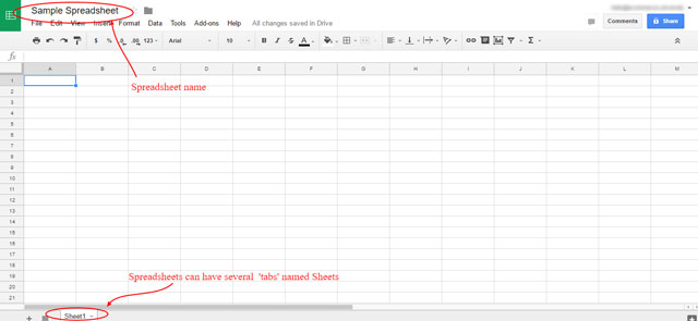
This very valuable tool, completely eliminated the need to physically write data and calculate values using a pen and paper. But what does it do? Here are some of it’s functions.

You can perform calculations with various formulas and functions, generate charts, pivot tables, filters or gather data automatically online even when it’s not open.
It allows you to create, edit or share spreadsheets from any device anywhere, even when you’re offline.
You can work simultaneously with your colleagues, see the changes as they make them, chat or comment in real time.
Your files will stay safe even if your computer dies because it saves changes automatically and everything’s stored in your Google Drive.

Whether you need to compile a report based on the existing data, keep track of your statistics or show your progress and results, make an inventory of all products – all you need is a web browser and a Google account. It’s that easy.

Now that you know how it looks like and what it does, let’s learn how to name and store the spreadsheets properly.

Naming Files and How Drive Works With Tags, Not Folders

Google Spreadsheets is a part of your Google Drive, which is an entire suite of products.

It is a storage and synchronisation online tool and besides Google Spreadsheets, it also has Google Doc, Slides and Forms, among some others, as well.

This is a short intro about Google Drive from the Google YouTube channel.

Just the same as spreadsheets, you can create your documents and slides using Google Drive tools. They are stored on your cloud drive, so you can share them, save them or even delete them.

But first of all – you have to name your files.

When naming files, people quite often use general terms such as sample, FAQs, article, curriculum vitae, tracking, project etc. instead of the names of specific projects they’re working on.

For example:

Bad filename: “statistics”

Good filename: “ 2014 Monthly Sales Statistics Report for Gazebos Australia”

Those “statistics” could be about your blog, about eCommerce store visitors or your sales, revenues and leads. But, that’s not transparent from the file’s name.

On the other hand, the second filename is much more ‘searchable’. If you try and search the file names by “monthly sales”, or “statistics report”, this file will end up in your search results.

Bad filename: “schedule”

Good filename: “Blog 2017 Monthly Editorial Schedule for Gazebos Australia”

“Schedule” could be any schedule! There could be dozens of files with that name.

This means that a person would be forced to open up several spreadsheets before finding the one they need.

The second name gives a much better idea about the content of the file.

Most people don’t think through these file names because they create folders. The person who named their file “schedule”, probably put it in a folder by the name “Gazebos Australia Blog 2017”. And if you opened that folder and found the file named “schedule” things would be a lot clearer.

Right? Wrong!

Why is it such a bad idea to count on your folder names to help you find the files you need?

Those folders actually don’t work the way you think they do because Google Drive works with tags, not folders.

In other words, folders in Google Drive are NOT folders although they look like they are.

They are the author’s personal non-transparent tags. This means that not everyone can see where a certain document is saved (without the link to it) or has the insight into how you’ve structured all of your content.

You can structure it very easily, by using your tags. Here is how you can move around your spreadsheet within your Drive, in just a couple of clicks:

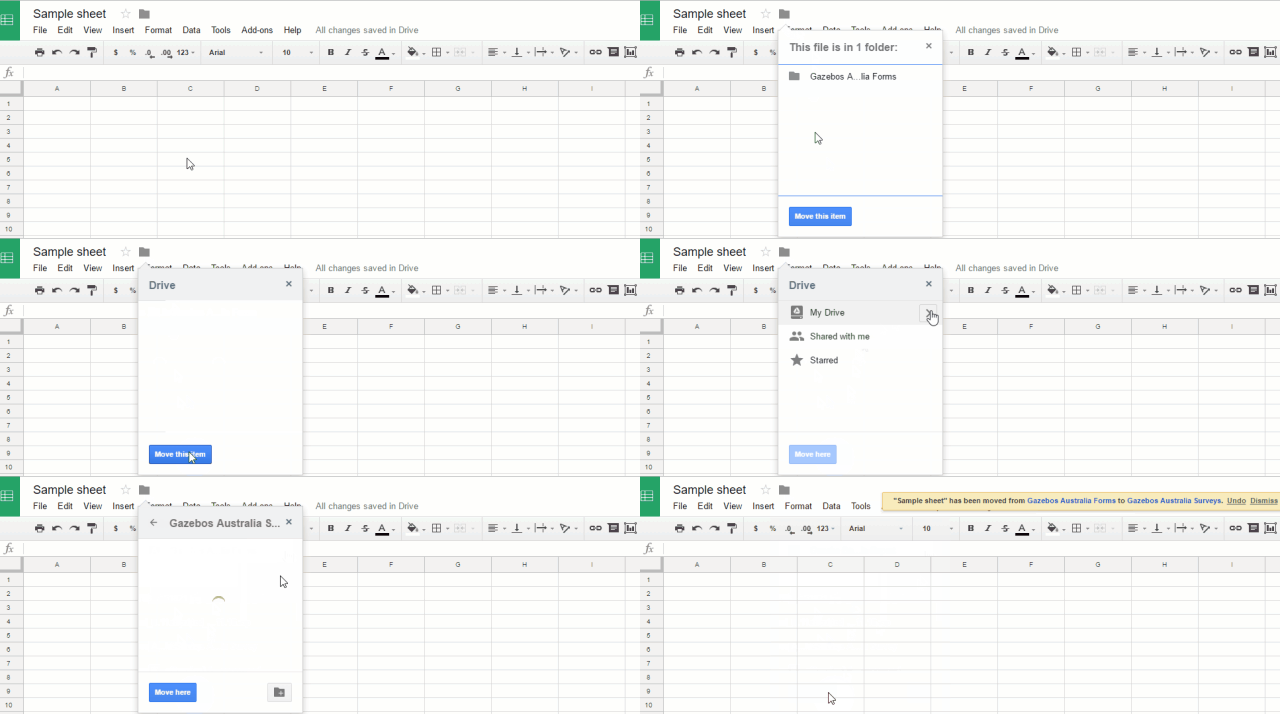
On your own Drive, your file will be stored in a folder-like place and it will make sense to you.

However, if you share it with somebody, the file will not ‘carry’ the folder name with it – it will end up in the “Shared with me” folder of their Drive.

Together with ALL the other files anybody shared with them, ever!

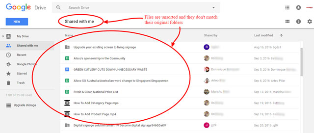
As you can see in the case of Gazebos Australia, these files are not sorted and they are not in their appropriate folders.

The only way for others to find your document is to search the Drive. Then they have to know how you have named it.

For instance, if you name a document A List of Branches without using the store name, or the website name, or what sort of branches they are (office or tree?) and what’s in that document, there’s no chance for someone else to find it. You see?

That’s exactly why you should use project names. Moreover, very long, precise names are welcome e.g. Gazebos Australia Monthly Statistics Tracking Report. If the other words are unknown or forgotten, using only the word “report” everyone has half a chance of finding this document.

If perhaps, your colleagues have to work on the same file as you, or to track it down for some reason, or you have to share a document with them, you should be aware that no one can see somebody else’s folders and how somebody’s content is structured.

Newbies are usually those unaware of this crucial fact. That’s why it’s super important to always make your file names searchable and meaningful.

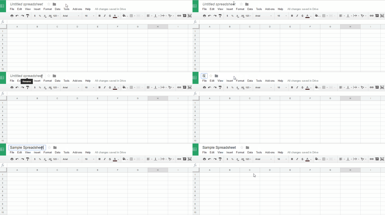
To name a file, just click to the “Untitled spreadsheet” and start typing.

Creating Sheets – Renaming, Copying, Duplicating and Hiding

When creating a new spreadsheet, you can make a new blank spreadsheet, or use some of the templates. It only takes three clicks to do so.

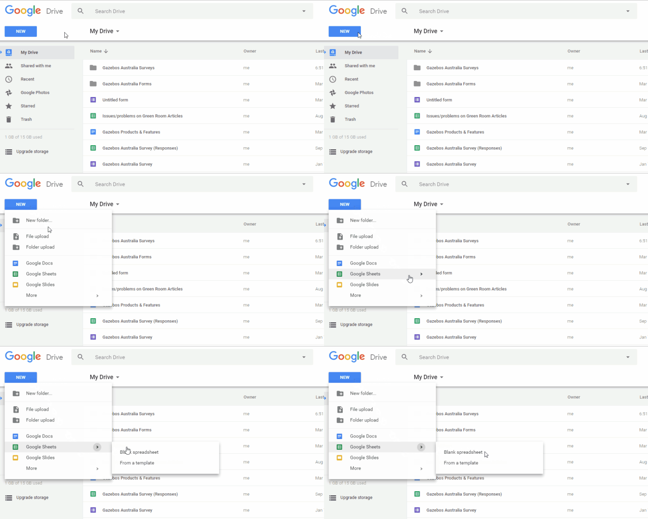
Once you do that, you have created a new file – a spreadsheet. Within that file, you have one or more sheets.

Sheets to a spreadsheet are like pages to a notebook.

Your new spreadsheet will have one sheet by default. This sheet is in a form of a tab, and you will find it in the bottom, left corner of your spreadsheet.

However, you can add more of these sheets by clicking on the “+” symbol on the left. Just like you can open a new tab on your browser, you can make many sheets within a spreadsheet.

You can add as many sheets as you like and you can manipulate them in many useful ways.

By right-clicking on the sheet’s name, you are able to:

Rename a sheet
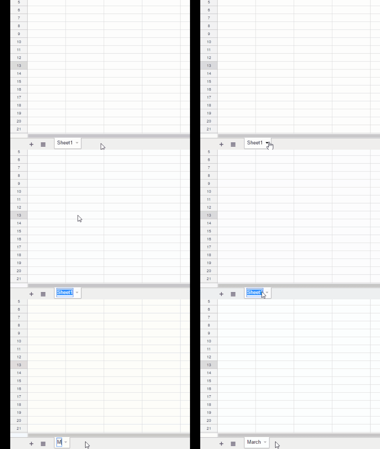
In this example, you can see how the default name “Sheet1” is being changed into the name “March”. If you are making some sort of an annual report and you use one sheet for every month, this is exactly how you’d do it.
Duplicate your sheet
For example, if you want to do lots of different calculations and you think you’ll possibly make a mistake, you make a duplicate and use it as a working file. You can always go back to your original sheet, which will remain intact.
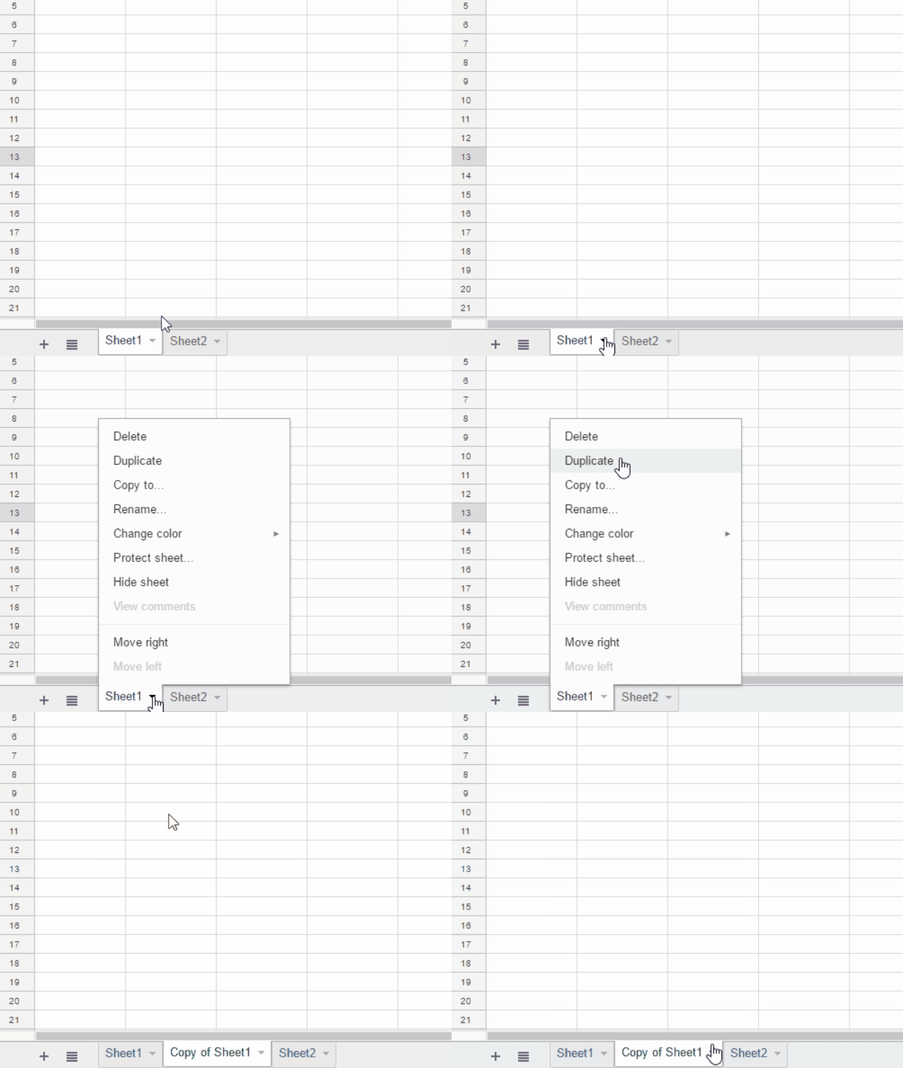As you can see, this will make the same copy of the sheet within the same document. If your sheet’s name was “Sheet1”, your copy will be named “Copy of Sheet1” by default. Of course, you can change that.
Copy the sheet
If you use this function, your sheet will be copied into another spreadsheet. If we compare your spreadsheet to a notebook again, and the sheets to its pages, this would be as if you copied the page from one notebook to another.
So, the difference between duplicating and copying is:
– duplicating makes the copy of a sheet within the same spreadsheet
– copying makes a copy of the sheet into a completely different spreadsheet of your choice
Hide the sheet
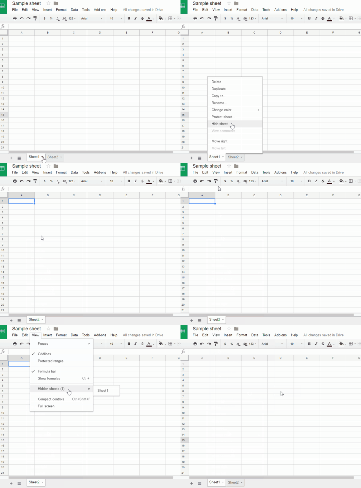
You can use this option if your sheet is not relevant anymore but you think you may need it later, or perhaps you just want it out of your way for the time being, without deleting it.
If you want the sheet to be visible again, go to “View” and find the “Hidden sheets” option. There, you will find all the hidden sheets listed, so you can choose which ones to make visible again.
Here, you can see how to hide “Sheet” and how to make it visible again.
These are the basic operations you can do with your spreadsheets and sheets. Now, it is time to learn how to properly input your data in those sheets, so you can do some really useful calculations.

Using Numbers, Not Letters to Ensure Accurate Calculations

First of all, when you want to do calculations with certain data, be careful to put in numbers into cells, NOT letters, a spacebar, a comma or any other character that’s not a number because the software cannot recognise it.

For example, if you try to calculate a sum of all the numbers of the column, let’s say they are the numbers of orders, all you need to do is use the SUM option, select the entire column and hit enter.

If you change the value of a cell into something other than a number, you will get a wrong result. Like this:

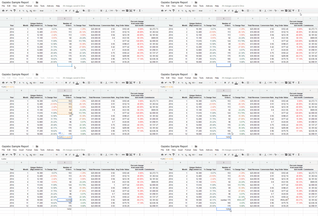
In our example, the SUM is 1432. However, if you change one cell and type in anything else besides a number, the formula will ignore it and make a calculation without it. In this case, it shows a wrong sum of 1262.

Even putting a space bar between numbers renders that number unrecognisable for the spreadsheet functions, e.g. 33000 – good; 33 000 – bad.

As a result, it won’t work out the SUM or AVERAGE, but show an error (#DIV/0) instead.

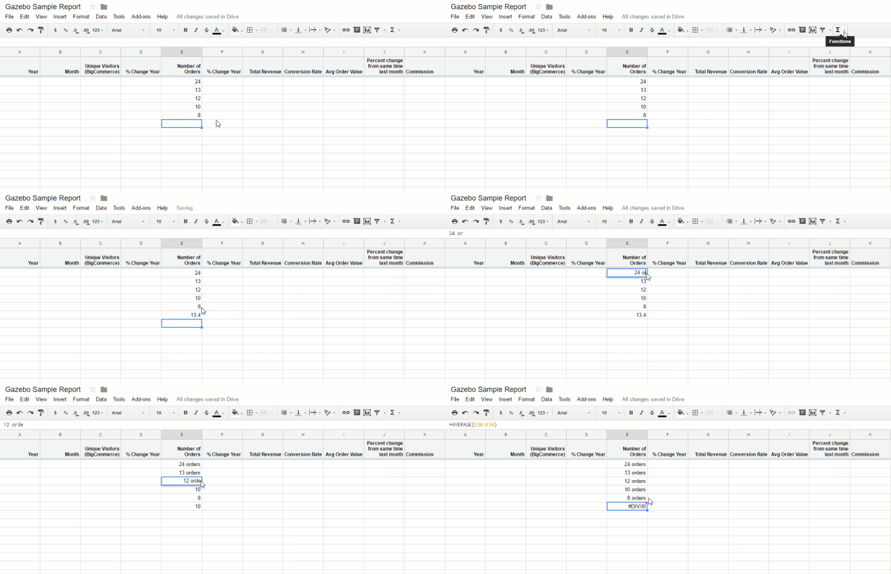
Here is another example from an actual spreadsheet. Firstly, the spreadsheet is used to calculate the average number of orders. It works well when only the numbers are put in the column.

However, if you try to write in “24 orders” instead of just “24”, the formula will ignore the cell and calculate the average from the remaining numeric values.

When it runs out of numbers, the spreadsheet reports the error #DIV/0.

Using Formatting for Better and More Efficient Communication

Good formatting means good communication whereas bad formatting means poor communication. Not only should you learn the mechanics of e.g. how to add in a line, but you should know how to be subtle. It’s acceptable to use a little bit of formatting but be careful not to go nuts about it.

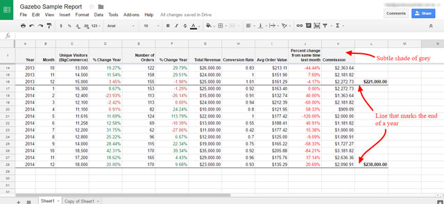
Here is a good example of a nicely and subtly formatted spreadsheet:

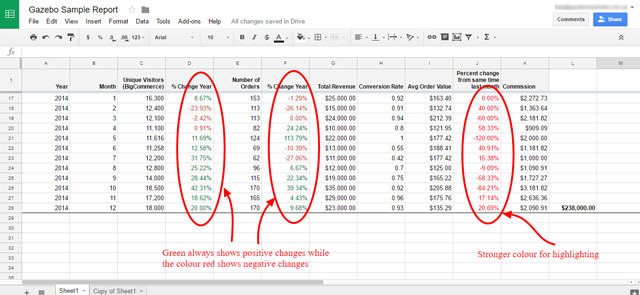
There are no background colours, different font shapes, sizes and colours. All the data is clearly visible and very easy to read. Good formatting helps you skim through the spreadsheet for the most important information without distracting you.

The spreadsheet looks professional, doesn’t it? This is the type of formatting that you need to avoid:

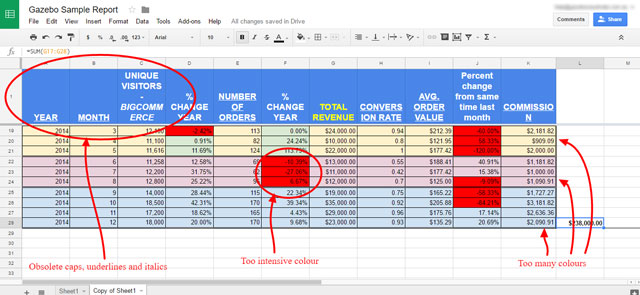
Too many colours are very distracting. They are not well-chosen and they are not used for emphasis – they are just everywhere. The same goes for the fonts.

If you take a quick look at this sheet, what would you say – what catches your attention first?

The answer is probably – everything! And you probably gave that answer after a few seconds of consideration. Everything on this spreadsheet screams for attention.

If you emphasise everything – you haven’t emphasised anything!

Use Subtle Lines and Background Colours

To denote e.g. the end of a period (a year) within a table, you can put a line in or make it stand out just a little bit by colouring it in e.g. a light grey. Keep in mind, black on white is clean and the easiest thing to read and comprehend.

On the other hand, using different dark and light colours, shades, fonts, ~~lines~~, different SiZeS, spacebars etc. makes your document really messy-looking.

Moreover, using CAPITALS in addition to this means you are shouting. NO SHOUTING, please!!! ?

Here is an example how all that excessive formatting looks in a spreadsheet:

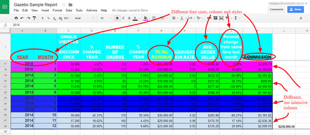
Google spreadsheet with different colours and formatting

All this means your layout (formatting) is poor and too many elements, colours, sizes and pieces of information are competing for your attention.

To say it again – If everything is shouting, then nothing stands apart.

In other words, the saying “Less Is More” is very much applicable when it comes to formatting. Therefore, every time when you ask yourself if you need to add an extra colour, line or border to your spreadsheet, the answer is probably – if you have to ask – no.

Use Conditional Formatting for Emphasis

You don’t have to format your spreadsheet all by yourself. You can create some rules of formatting that the spreadsheet will apply automatically. That is called conditional formatting. In other words, you are setting a condition and if that condition is met – certain formatting is applied.

For example: You can make a rule that orders your sheet to colour the numbers in the cell green if their value is less than 20,000.

Conditional formatting is very useful in cases when you want to draw attention to a certain piece of information within your spreadsheet.

For example: If you are making a report about an eCommerce store and you want to compare it with the last year’s results, you can use conditional formatting to help you get a better picture about your progress.

You can make it by setting a conditional formatting rule to colour all the negative results in red and all the positive results in green. Visually, it can help any eCommerce owner to get a general idea if they are doing well, or not in comparison to the previous year.

If they want to know all the details – they are right there, but the proper use of conditional formatting and well-chosen colours paint a bigger picture that is obvious right away. Another reason to learn conditional formatting is – it saves time!

You don’t have to waste your time going individually from one cell to another and then colouring it or changing the background. It does that for you automatically.

Also, you can format massive amounts of data, all at once, not to mention the fact that it reduces errors in formatting to a minimum.

In other words, if you set a conditional formatting rule to colour negative values red – it will always be coloured in the same shade of red and it will never miss a cell in your assigned range, or accidentally colour a positive cell in that colour.

Now that it’s clear what it does and why you need it, let’s learn how to actually do it. Let’s do the conditional formatting from the example we mentioned above. We are going to select a range of cells (column F) and set a conditional formatting rule to colour all the negative values red and all the positive ones green:

Firstly, you need to set the range of cells you want affected by conditional formatting (you can apply it to the entire sheet, a whole column or just a couple of cells).

Once you set the range, open Format and pick Conditional formatting. That opens a dialog in which you choose a condition (in our case that the cells with values less than 0 should be affected) and the format (What to do with these cells? Colour them red.)

Again, the rules about subtle and effective formatting apply: it looks much better if the colours are not too intensive and if background is left white.

Hide Rows and Columns for Better Visibility

Sometimes it’s easier to comprehend the content of a document if you hide all the extra stuff. It’s very simple: select the row(s)/column(s) you want to hide, right-click a row/column heading and choose the option hide row/column from the drop-down menu.

To make them appear again, click on the little arrows you can see below.

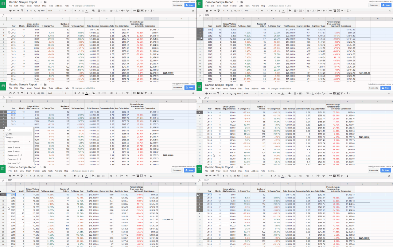
hiding rows and columns in Google spreadsheet

When something is hidden, it does NOT mean it’s deleted. The same procedure can be applied to insert or delete or move rows/columns, just choose those options from the drop-down menu that appears when you right-click.

Freeze the Top Row for Easier Navigation

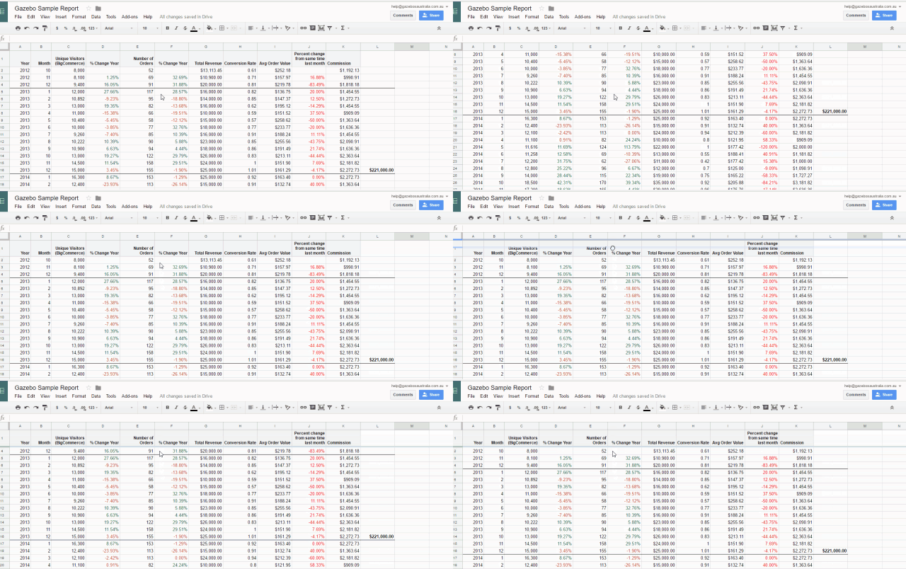
If you want your top row (or more rows) to stay fixed while you scroll down your worksheet, click View in the toolbar, then hover the mouse over Freeze and select the desired number of rows to freeze from the drop-down menu.

You can also “grab” the line shown below and drag it where you want.

Using the SUM and the Other Formulas

Although this is such basic stuff, for some reason a lot of people don’t know how to do it. When you have a bunch of numbers lined up correctly, you can select them and add them all up.

In simple words, you can use your spreadsheet a bit like a calculator. It can do all the basic operations like adding, subtracting, multiplying and dividing numbers.

If you want to add numbers, you will use the SUM formula, but you can follow the same steps to choose many other functions as well, such as:

AVERAGE to find the average of a range of cells you select
COUNT counts a value in a range of cells
MAX finds the highest value in a range of cells
MIN finds the lowest value in a range of cells and others

using sum and other Google spreadsheet formulas

The functions might be different, but the way you use them is the same. You need to:

Select the cell in which you want your result to be shown
Choose the function from the menu
Select the range of cells on which you want the operation to be applied
Hit the Enter key on your PC or the Return key on your Apple

Another way of doing the SUM is to type the formula into the result cell (using =) and then select the range of cells you want to add up, or manually type them.

The same steps are followed when using the AVERAGE option, as well. You need your result cell, your range of cells, but instead of SUM, you will use AVERAGE.

Calculating Percentages to Monitor the Ecommerce Store Progress

You need to know how to use your spreadsheets to calculate the percentages, because that will help you monitor the progress of your eCommerce store success.

For example, you need to make the formula that calculates whether your sales have gone up or down in comparison to the same month in the previous year. Not only that, but you can express that difference in percentages.

Moreover, now that you know how to use conditional formatting, why not colouring those cells red if your sales have dropped or green if they are increased?

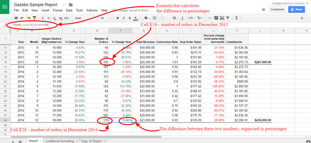
Let’s take a look at our example, one more time. The column E of this spreadsheet shows the number of orders for each month. We can see the results for the year 2013 and the year 2014.

If you want to keep track of your orders, it is very useful to be able to see if that number of orders increased or decreased in comparison to the same month of the previous year.

Even better – you can calculate the percentage of that increase or decrease. It is all about creating the right formula. It is a slightly more complicated SUM formula, but still a very basic calculation.

Let’s say the number of sales for the December 2013 is expressed in the cell E16. The number of sales for the December 2014 is in the cell E28.

E16 has the value of 155 while E28 has the value of 176. Obviously, there is an increase in the number of sales. More precisely, the increase is 9.68%, which is expressed in the cell F28.

How do we know? By creating a simple formula.

First, we pick the cell F28 to be our result cell. Then we type in the following formula:

=SUM(E28-E16)/E16*100%

You need to do such calculations because it’s helpful to know whether you’re (not) getting better at something. Calculating and monitoring percentages helps you see whether you are doing something right or not.

When you do the math in the calculation row of your Google sheet, it’s useful to double-check your work. Percentage Calculator is a fantastic, handy tool for checking your percentages.

Let’s use it to check our calculations from the example above:

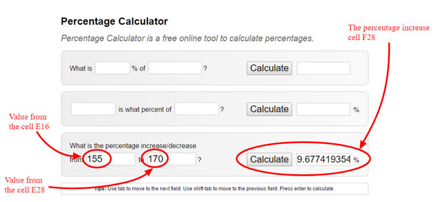
The cells in the spreadsheet have been formatted to round up the numbers to two decimals. That’s why the result in the spreadsheet is 9.68% and the Percentage Calculator shows 9.677419354%.

The formula works and the results are checked

In Summary

Google Spreadsheets is a common tool that so many eCommerce store owners use that you would hardly be considered for a job if you are a stranger to it. Knowing your way around this tool can get you hired and keep you hired.

Being able to create well formatted and useful reports and statistics presentations makes you look very professional and useful to the team.

You won’t be struggling with using such a common tool, and you’ll be able to jump in and manage data and deal with different sorts of analytics.

You can find more detailed information at G Suite Learning Center. These are just very basic things which are truly useful in any freelancer’s line of work. Everyone should know at least:

what Google Sheets are and how they work,
how to create, name, rename, delete, copy, duplicate or hide a sheet,
how to use subtle formatting to communicate effectively,
how to hide rows and columns and freeze the top row
how to do basic calculations using the formulas.
how to calculate, check and use percentages to monitor eCommerce store progress